Fast Fourier Transforms (FFT)

Image processing uses processes called "Transforms" to manipulate and compress images. These "transformations" include the Fourier Transform (FT), Walsh Transform, Hadamard Transform, Discrete Cosine Transform (DCT), Haar Transform, and Slant Transform. Of all these transforms, the best known is the Fourier Transform. Deriving the other transforms is usually analogous to the derivation of the FT.

Essentially, the Fourier Transform maps a given function f(x) from the Spatial Domain (of x) into the Frequency Domain (u) using the Fourier Function F(u). This is useful for implementing frequency filters and other processing techniques. For this transformation to work, f(x) must be integratable and continuous over the range (+infinity,-infinity).

The Fourier Transform of f(x) (in one dimension) is given by:

F(u) = ∫ f(x)e^-i2*π*ux ∂x

where e represents the natural log and i is the square root of (-1) and thus F(u) is usually a complex function.

When given the Fourier Transform, the original function can be derived using the formula:

f(x) = ∫ F(u)e^-i2*π*ux ∂u

When graphed, the spectrum of F(u) is usually graphed. The spectrum is defined as (here with "|" being used in the sense of "absolute value" notation):

|F(u)| = (R² + I²)^0.5

or the absolute value or magnitude of F(u) using the length of the hypotenuse of the complex number when graphed on the Argand plane. In the same way as the one dimensional Fourier Transform, a two dimensional function can also be derived using:

F(u,v) = ∫∫ f(x,y)e^{-i2*π*(ux+vy)} ∂x∂y

and its inverse Fourier Transform:

f(x,y) = ∫∫ F(u,v)e^i2π(ux+vy) ∂u∂y

Resolution of Complex numbers in a form suitable for computer manipulation involves invoking Euler's Formula of the form:

e^-i2π*ux = cos(2π*ux) - i*sin(2π*ux)

Discrete Fourier Transforms

Because computers cannot handle continuous functions, the Fourier Transform is "discretized" over some arbitrary range using the formula:

F(u) = (1/N)∑_x=0^N-1 f(x)e^-i2π*ux/N

where (1/N) becomes a scaling factor for the total of N points in the set. The two dimensional Discrete Fourier Transform (DFT) is derived analogously.

Fast Fourier Transforms

One problem with Discrete Fourier Transforms is their computation cost. A one dimensional transform takes n² cycles to compute: one cycle for each value of x and one for each value of u (since u=x). This cost is even more excessive for two dimensional transforms where we need to cycle through each value of x,y,u and v for a O(n)=n⁴. These costs make Fourier Transforms difficult to compute for all but very small images (where x is very small).

Fortunately, this computation cost can be reduced using a technique called the Fast Fourier Transform (FFT). Information, discussions, and algorithms for the FFT are available throughout the internet and a selection of links is provided below. Using FFT, the computational effort required to derive the one dimensional FT is now n*log₂n and for the two dimensional FT, O(n)=n²log₂n--a very dramatic improvement.

Results

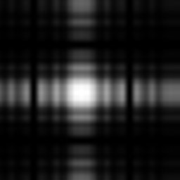
To illustrate what Fourier Transforms look like, the left hand image is the image of f(x), and the image on the right its respective Fourier Transform. The 32 and 64 bit images were created using the Discrete Fourier Transform using the code supplied. The 256 bit images were created using the Fast Fourier Transform algorithm. In all cases, the Fourier Transforms were rotated 90 degrees around the origin to shift the image to the center of the display. Note: All the images have been scaled to the same size for consistency of appearance.

Spatial images and their Fourier transforms
Spatial Images	Fourier Transforms
A square in a 32x32 pixel image and its associated Fourier Transform. (Any ghosted images in the white square was caused by JPEG compression. The square should be completely white.)
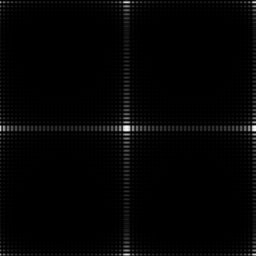
A square in a 64x64 pixel image and its associated Fourier Transform.
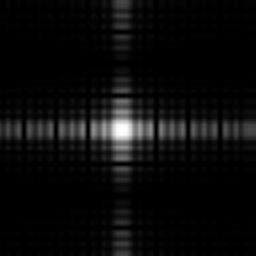
A square in a 256x256 pixel image and its associated Fourier Transform.
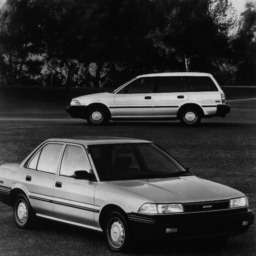
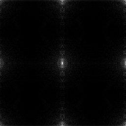
A photograph in a 256x256 pixel image and its associated Fourier Transform.

As can be seen from the transforms, the image is a sparsely populated set of data points. Compression is possible by measuring a radius from the middle and then truncating all points outside of the resulting circle. This compression will also lose some higher frequency detail. Alternatively, truncating data points within the middle of the image will result in a loss of low frequency components of the image.

The accompanying source code is copyright the author and all rights are reserved. Please do not reproduce this code for any projects, publications, or assignments without the express permission of the author.

Code

My code (in C) for Fourier Transforms is available.

main.c: The main program controls the file I/O, image parsing, conversion to complex numbers, and image representation functions. Note that the size of the image is hard coded as precompiler directives. The code could also receive the image size as a parameter and utilize calloc calls to create the necessary arrays. Verbose output is available by defining _DEBUG_ as a precompiler directive.
img.h: Global variables and struct definitions and functions supporting Complex number calculations.
fft.h: The header file for the Discrete Fourier Transform, Fast Fourier Transform and supporting functions. The reverse function performs a bit-wise reversal of the image array's subscripts. The bit_print function is courtesy of the Al Kelley and Ira Pohl book A Book on C.
fft.c: The source code for the functions contained in fft.h

Other References

Fast Fourier Transform [1]

Language:

Archive:

fft.zip [3]

Main program

Project Name:

Fast Fourier Transforms (FFT) [4]

Filename:

main.c

Language:

Summary:

Main procedure for the Fast Fourier Transform algorithm

Code:

#include <stdio.h> #include <math.h> #include <stdlib.h> /******************************************** ** This program determines the Fast Four- ** ** ier Transform (FFT) of a supplied image.** ** The program does this by calling the ** ** routines referenced in the fft.h file. ** ** ** ** Author: Daryle Niedermayer ** ** Date: Oct 5, 1999 ** ** ** ** Credits: Derived from the template ** ** supplied by Xue Dong Yang ** ** Oct 2, 1999 ** ** ** ** To see the FFT run though its procedure ** ** define _DEBUG_ ** ********************************************/ #undef _DEBUG_ /******************************************** ** ROWS and COLS must be defined for the ** ** correct image size. ** ********************************************/ #define ROWS 64 #define COLS 64 /******************************************** ** This same procedure can be used to gen ** ** erate either the FFT or DFT algorithms. ** ** Define either _FFT_OPT_ or _DFT_OPT_ ** ** here. ** ** _FFT_OPT_ is the default. ** ********************************************/ #define _FFT_OPT_ #ifdef _DFT_OPT_ #undef _FFT_OPT_ #else #define _FFT_OPT_ #undef _DFT_OPT_ #endif /******************************************** ** Other files and definitions to include ** ********************************************/ #include "img.h" /* Assume it is at the current directory */ #include "fft.h" /* Fast Fourier Transform routines */ unsigned char in_buf[ROWS][COLS]; /* Buffer for the input image */ unsigned char out_buf[ROWS][COLS]; /* Buffer for the output Fourier spectrum image */ main(argc, argv) int argc; char **argv; { FILE *fin, *fout; int i, j, n; /* i and j are loop counters */ /* n is the log(N) of the */ /* sample size. */ float max, scale_factor; /* used for scaling the im- */ /* ages brightness. */ COMPLEX *ft; /* pointer to the array con- */ /* taining the results of */ /* the ft. */ COMPLEX F_buffer[ROWS]; /* Buffer of complex numbers */ /* to hand off to FT function*/ int half_width, half_height; unsigned char swap_buf[ROWS][COLS]; /* Shifted image for output */ /* Check the number of arguments in the command line. */ if (argc != 3) { fprintf(stderr, "Usage: %s in.img out.img\n", argv[0]); exit(1); } /* Open the input image file */ if ((fin = fopen(argv[1], "rb")) == NULL) { fprintf(stderr, "ERROR: Cann't open input image file %s\n", argv[1]); exit(1); } /* Open the output image file */ if ((fout = fopen(argv[2], "wb")) == NULL) { fprintf(stderr, "ERROR: Cann't open output image file %s\n", argv[2]); exit(1); } /* Load the input image */ if ((n=fread(in_buf, sizeof(char), ROWS*COLS, fin)) < ROWS*COLS*sizeof(char)){ fprintf(stderr, "ERROR: Read input image file %s error)\n", argv[1]); exit(1); } /* Convert the real image into complex image first. */ for (i=0; i<ROWS; i++) for (j=0; j<COLS; j++) { F[i][j].r = (float)in_buf[i][j]; /* The real part = input image */ F[i][j].i = 0.0; /* The imaginery part = 0 */ } /* ========================= PASS 1 ============================== Applying the 1D FFT function to each columun of the input image, and save the intermediate results into a temparory array F1. =============================================================== */ for (j=0; j<COLS; j++) { /* Copy a column from array F into the temporary vector TF*/ for (i=0; i<ROWS; i++) { F_buffer[i].r = F[i][j].r; F_buffer[i].i = F[i][j].r; } /* Call the corresponding function to compute the Fourier transform depending on whether the _DFT_OPT_ or _FFT_OPT_ flag is set */ #ifdef _DFT_OPT_ ft = DFT(F_buffer,ROWS); #else ft = FFT(F_buffer,ROWS); #endif /* Copy the returned result into a temporary array F1 */ for (i=0; i<ROWS; i++) { F1[i][j].r = ft[i].r; F1[i][j].i = ft[i].i; } } /* ========================= PASS 2 ============================== Applying the 1D FFT function to each row of the intermediate results, and save the result back into array F. =============================================================== */ for (i=0; i<ROWS; i++) { /* Copy a row from array F1 into the temporary vector TF*/ for (j=0; j<COLS; j++) { F_buffer[j].r = F1[i][j].r; F_buffer[j].i = F1[i][j].r; } /* Call the corresponding function to compute the Fourier transform depending on whether the _DFT_OPT_ or _FFT_OPT_ flag is set */ #ifdef _DFT_OPT_ ft = DFT(F_buffer,ROWS); #else ft = FFT(F_buffer,ROWS); #endif /* Copy the returned result back into array F */ for (j=0; j<COLS; j++) { F[i][j].r = ft[j].r; F[i][j].i = ft[j].i; } } /* Compute the Fourier spectrum |F(u,v)| and save it into the output image buffer out_buf. Note that proper scaling for the values is needed in order to obtain a reasonably bright image. Refer to the discussion on page 92, the last paragraph. */ max = 0; for (i=0; i<ROWS; i++) { for (j=0; j<COLS; j++) { if (complex_mag(F[i][j]) > max) max = complex_mag(F[i][j]); } } #ifdef _DEBUG_ printf ("The min and maximum values are: %f and %f \n",min,max); #endif scale_factor = 255/(log(1 + max)); for (i=0; i < ROWS; i++) { for (j=0; j < COLS; j++) { out_buf[i][j] = (unsigned char) scale_factor*(log(1 + complex_mag(F[i][j]))); } } /* Swap sectors of the image to reposition the image to the center of the screen. */ half_height = (int)ROWS/2; half_width = (int)COLS/2; for (i=0; i<half_height; i++) { for (j=0; j<half_width; j++) { swap_buf[half_height+i][half_width+j] = out_buf[i][j]; swap_buf[i][j] = out_buf[(half_height-1)-i][(half_height-1)-j]; swap_buf[i][j+half_width] = out_buf[(half_height-1)-i][j]; swap_buf[half_height+i][j] = out_buf[i][(half_width-1)-j]; } } /* Save the output Fourier spectrum image */ if ((n=fwrite(swap_buf, sizeof(char), ROWS*COLS, fout)) < ROWS*COLS*sizeof(char)) { fprintf(stderr, "ERROR: Write output image file %s error)\n", argv[1]); exit(1); } fclose(fin); fclose(fout); }

Header file for complex number structures and methods

Project Name:

Fast Fourier Transforms (FFT) [4]

Filename:

img.h

Language:

Summary:

This file is courtesy of Dr. Xue Dong Yang

Code:

/* ======================================= * * IMAGE FORMAT DEFINITIONS * * Dr. Xue Dong Yang * ======================================= */ #include <stdio.h> #include <math.h> #ifndef ROWS #define ROWS 256 #endif #ifndef COLS #define COLS 256 #endif unsigned char in_img[ROWS][COLS]; /* Input raw raster image */ unsigned char out_img[ROWS][COLS]; /* Output raster image */ typedef struct complex { float r,i; /* Real and imaginery parts */ } COMPLEX; COMPLEX F[ROWS][COLS]; /* Arrays used FFT computation */ COMPLEX F1[ROWS][COLS]; COMPLEX TF[COLS]; /* Some functions for complex arithmetics */ COMPLEX complex_plus(c1, c2) COMPLEX c1, c2; { COMPLEX c; c.r = c1.r + c2.r; c.i = c1.i + c2.i; return( c ); } COMPLEX complex_minus(c1, c2) COMPLEX c1, c2; { COMPLEX c; c.r = c1.r - c2.r; c.i = c1.i - c2.i; return( c ); } COMPLEX complex_times(c1, c2) COMPLEX c1, c2; { COMPLEX c; c.r = c1.r*c2.r - c1.i*c2.i; c.i = c1.r*c2.i + c2.r*c1.i; return( c ); } int complex_print(COMPLEX c) { printf("[%f,%f]", c.r, c.i); return (1); } double complex_mag(COMPLEX c) { return (sqrt(pow(c.r,2) + pow(c.i,2))); }

Fast Fourier Transform Header file

Project Name:

Fast Fourier Transforms (FFT) [4]

Filename:

fft.h

Language:

Code:

/******************************************** ** Function prototypes and header infor- ** ** mation for the "fft.c" file. ** ** ** ** Author: Daryle Niedermayer ** ** Date: Oct 5, 1999 ** ********************************************/ #include <math.h> #include <stdlib.h> #include <stdio.h> #include <limits.h> #ifndef _FFT_ #define _FFT_ /*********************************************** ** unsigned char: the integer to convert ** using bitwise operators. ** int: the size of the passed integer in bits ***********************************************/ unsigned char reverse(unsigned char, int); /*********************************************** ** DFT is a one dimensional standard Fourier ** Transform based of the FT definition. ***********************************************/ COMPLEX *DFT(COMPLEX[], int); /*********************************************** ** FFT receives parameters: ** int: the dimension of the given array ** where array is of size int*int ** COMPLEX**: a pointer to a two dimensional ** array of complex numbers containing ** the initial image. ***********************************************/ COMPLEX *FFT(COMPLEX[], int); #include "fft.c" /*********************************************** ** int: the integer to print out in bits ***********************************************/ void bit_print(int); #endif

Fast Fourier Transform Source File

Project Name:

Fast Fourier Transforms (FFT) [4]

Filename:

fft.c

Language:

Code:

/******************************************** ** FFT: the subroutine to calculate and ** ** return the 1D-FF transform of a input- ** ** ted image. ** ** ** ** reverse: a subroutine to take an ** ** integer of n bits and reverse it from ** ** high-endian to low-endian order. ** ** ** ** Author: Daryle Niedermayer ** ** Date: Oct 5, 1999 ** ** Credits: Thanks to Paul Bourke for ** ** his contribution and explan- ** ** ations ** ** (http://www.swin.edu.au/ ** ** austronomy/pbourke) ** ********************************************/ /******************************************** ** REVERSE: Strategy... ** ** using a single pass, take the most sig- ** ** nificant and least significant bits and ** ** switch them. For this purpose, leftbit ** ** and rightbit are temporary values of ** ** the bits requiring switching, and left- ** ** place and rightplace are the positions ** ** of these bits in the integer. ** ********************************************/ unsigned char reverse(unsigned char input, int n) { unsigned char leftbit, rightbit, output; int i, leftplace, rightplace; leftplace = n-1, rightplace = 0; output = 0; while (leftplace >= rightplace) { /* Create bit masks for left and right places */ leftbit = 1 << leftplace; rightbit = 1 << rightplace; /* Use masks to get the value of the bits */ leftbit = input & leftbit; rightbit = input & rightbit; /* Switch the places for these bits */ leftbit = leftbit >> (leftplace - rightplace); rightbit = rightbit << (leftplace - rightplace); /* Use masks to insert values into input */ output = output | leftbit; output = output | rightbit; /* Increment/Decrement placement holders */ leftplace--; rightplace++; } /* while (leftplace > rightplace) */ return output; } /******************************************** ** DFT calculates the 1D-Discrete Fourier ** ** Transform using the definition of a ** ** Fourier Transform: ** ** F(u)=(1/N)Sum[from x=0 to N-1]f(x)exp^ ** ** (-j2*pi*ux/N) ** ********************************************/ COMPLEX *DFT(COMPLEX F[], int N) { int u, x; double cosarg = 0; double sinarg = 0; double W; COMPLEX *ft; COMPLEX tmp; for (u=0; u<N; u++) { /* Zero out the temporary array as we go */ TF[u].r = 0; TF[u].i = 0; W = 2*PI*u/N; for (x=0; x<N; x++) { tmp.r = cos(W*x); tmp.i = -1*sin(W*x); /**************************************************** ** To find the sums in complex form, we must ** cross-multiply f(x) with the cos and sin functions ** from Euler's Formula: ** TF.r*(cosarg - sinarg) + TF.i*(cosarg - sinarg) = ** TF.r*cosarg - TF.i*(sinarg) = TF.r ** TF.i*cosarg + TF.r*(sinarg) = TF.i ****************************************************/ TF[u] = complex_plus(TF[u],(complex_times(F[x],tmp))); } TF[u].r = TF[u].r/N; TF[u].i = TF[u].i/N; } ft = TF; return ft; } /******************************************** ** FFT calculates the 1D-FFT of a complex ** ** array passed into the function. The ar- ** ** ray is expected to be of size N. ** ********************************************/ COMPLEX *FFT(COMPLEX F[], int N) { int i, M, j, k, u, i1, i2; COMPLEX F2[N]; COMPLEX Half, W2M; int new_index[N]; int n=(int) log(N) / log(2); #ifdef _DEBUG_ printf("The value of n is: %d\n",n); #endif Half.r = 0.5; Half.i = 0.0; /***************************************** ** Reverse the array indexes *****************************************/ for (i=0; i<N; i++) { new_index[i] = reverse(i,n); } /***************************************** ** Rearrange array elements *****************************************/ for (i=0; i<N; i++) { TF[new_index[i]] = F[i]; } /***************************************** ** Begin decomposing the array into ** subgroups. *****************************************/ M = 1; /* The initial length of subgroups */ j = N/2; /* The number of pairs of subgroups */ /** Begin successive merges for n levels */ for (i=0; i<n; i++) { /** Merge pairs at the current level */ for (k=0; k<j; k++) { i1 = k*2*M; /* Start of first group */ i2 = (k*2+1)*M; /* Start of second group */ #ifdef _DEBUG_ printf("Cycling through k=%d... i1 and i2 = %d and %d...\n",k,i1, i2); #endif for (u=0; u<M; u++) { W2M.r = cos(PI*u/M); W2M.i = -sin(PI*u/M); #ifdef _DEBUG_ printf("M is currently: %d\n",M); printf("Cycling through u=%d...\n",u); printf("Cycling through i=%d... W2M=%f\n",i,W2M); #endif /* Calculate the values for the first set of numbers */ F2[u] = complex_times(Half,(complex_plus(TF[i1+u], \ complex_times(TF[i2+u],W2M)))); /*Calculate the values for the second set of numbers */ F2[u+M] = complex_times(Half,(complex_minus(TF[i1+u], \ complex_times(TF[i2+u],W2M)))); TF[i1+u] = F2[u]; TF[i1+u+M] = F2[u+M]; #ifdef _DEBUG_ printf("F2[%d] is: ",u); complex_print(F2[u]); printf("\n"); printf("F2[%d] is: ",u+M); complex_print(F2[u+M]); printf("\n"); printf("TF[%d] is: ",i1+u); complex_print(TF[i1+u]); printf("\n"); printf("TF[%d] is: ",i1+u+M); complex_print(TF[i1+u+M]); printf("\n"); #endif } } M = 2*M; j = j/2; } return TF; } /******************************************** ** bit_print is a little utility to print ** ** out an integer bitwise for debugging ** ** purposes. ** ********************************************/ void bit_print(int a) { int i; int n = sizeof(int) * CHAR_BIT; int mask = 1 << (n - 1); for (i=1; i<=n; ++i) { putchar(((a & mask) == 0) ? '0' : '1'); a <<= 1; if (i % CHAR_BIT == 0 && i<n) putchar(' '); } printf("\n"); }