--Daryle Niedermayer, I.S.P., ITCP, PMP, B.A., B.Sc., M.Div., M.Ed.
December 1, 1998
Bayesian Networks are becoming an increasingly important area for research and application in the entire field of Artificial Intelligence. This paper explores the nature and implications for Bayesian Networks beginning with an overview and comparison of inferential statistics and Bayes' Theorem. The nature, relevance and applicability of Bayesian Network theory for issues of advanced computability forms the core of the current discussion. A number of current applications using Bayesian networks is examined. The paper concludes with a brief discussion of the appropriateness and limitations of Bayesian Networks for human-computer interaction and automated learning.
Inferential statistics is a branch of statistics that attempts to make valid predictions based on only a sample of all possible observations[1] [1]. For example, imagine a bag of 10,000 marbles. Some are black and some white, but of which the exact proportion of these colours is unknown. It is unnecessary to count all the marbles in order to make some statement about this proportion. A randomly acquired sample of 1,000 marbles may be sufficient to make an inference about the proportion of black and white marbles in the entire population. If 40% of our sample are white, then we may be able to infer that about 40% of the population are also white.
To the layperson, this process seems rather straight forward. In fact, it might seem that there is no need to even acquire a sample of 1,000 marbles. A sample of 100 or even 10 marbles might do.
This is assumption is not necessarily correct. As the sample size becomes smaller, the potential for error grows. For this reason, inferential statistics has developed numerous techniques for stating the level of confidence that can be placed on these inferences.
If we took ten samples of 100 marbles each, we might find the following results:
| Sample Number | Number of White Marbles |
Number of Black Marbles |
|---|---|---|
| 1 | 40 | 60 |
| 2 | 35 | 65 |
| 3 | 47 | 53 |
| 4 | 50 | 50 |
| 5 | 31 | 69 |
| 6 | 25 | 75 |
| 7 | 36 | 64 |
| 8 | 20 | 80 |
| 9 | 45 | 55 |
| 10 | 55 | 45 |
We are then in a position to calculate the "Standard Deviation" of these samples:
where x2 is the sum of the squares so that the equation is expanded to:
and n is the number of samples. In our example, the mean number of White marbles is ![]() .
.
We might be tempted to say that about 40% of the marbles are white, but we are unable to argue that point with any degree of certainty. Using equation 2 above, we determine that the Standard Deviation is 11.15. We must then determine the "Sample Error of the Mean" (where s=[sigma]):
The confidence we can put on our hypothesis that u=40 of the marbles are white is found using a standard statistical test called the "z-test":
Using a z-test table [3] [3] and our resulting z-value of -.4532, we find that 32% of the area of the normal curve would fall below this "z" value. In other words, in 32% of samples given ![]() ,
,  would be less than 38.4. Since the distribution is two-sided or "two-tailed" (i.e. the sample average could also be greater than the population average), we would also expect
 ![]() to greater than ((u-
to greater than ((u-![]() )+u=) 41.6 in another 32% of cases.
)+u=) 41.6 in another 32% of cases.
In summary, if we expect 40% of all marbles in the bag to be white, then a series of ten samples with only 38.4% of marbles being white would be expected in (100-64%=) 36% of the time. Clearly, the confidence we can place in our conclusion is not as good as it was on first glance. This lack of confidence is due to the high variability among the samples. If we took more samples or larger samples, our confidence in our conclusion might increase.
Classical inferential models do not permit the introduction of prior knowledge into the calculations. For the rigours of the scientific method, this is an appropriate response to prevent the introduction of extraneous data that might skew the experimental results. However, there are times when the use of prior knowledge would be a useful contribution to the evaluation process.
Assume a situation where an investor is considering purchasing some sort of exclusive franchise for a given geographic territory. Her business plan suggests that she must achieve 25% of market saturation for the enterprise to be profitable. Using some of her investment funds, she hires a polling company to conduct a randomized survey. The results conclude that from a random sample of 20 consumers, 25% of the population would indeed be prepared to purchase her services. Is this sufficient evidence to proceed with the investment?
If this is all the investor has to go on, she could find herself on her break-even point and could just as easily turn a loss instead of a profit. She may not have enough confidence in this survey or her plan to proceed.
Fortunately, the franchising company has a wealth of experience in exploiting new markets. Their results show that in 20% of cases, new franchises only achieve a 25% market saturation, while in 40% of cases, new franchises achieve a 30% market saturation. The entire table of their findings appears below:
| Percent of New Franchises achieving a given Market Saturation" | Percent of Franchises (Relative Frequency) |
|---|---|
| 0.10 | 0.05 |
| 0.15 | 0.05 |
| 0.20 | 0.20 |
| 0.25 | 0.20 |
| 0.30 | 0.40 |
| 0.35 | 0.10 |
| Total = 1.00 |
Our investor's question is simple: "What is the probability that my population will achieve a market saturation of greater than 25% given the poll conducted and the results found in other places?" In effect, she needs to determine the probability that her population will one of the 70% of cases where market saturation is greater than or equal to 25%. She now has the information she needs to make a Bayesian inference of her situation.
Bayes' Theorem, developed by the Rev. Thomas Bayes, an 18th century mathematician and theologian, was first published in 1763.[4] [4] Mathematically it is expressed as:
![]() (eq.6)
(eq.6)
where we can update our belief in hypothesis H given the additional evidence E and the background context c. The left-hand term, P(H|E,c) is known as the "posterior probability," or the probability of H after considering the effect of E on c. The term P(H|c) is called the "prior probability of H given c alone. The term P(E|H,c) is called the "likelihood" and gives the probability of the evidence assuming the hypothesis H and the background information c is true. Finally, the last term P(E|c) is independent of H and can be regarded as a normalizing or scaling factor.
In the case of our investor, P(H|c) is already known to be 0.40 so the Bayesian equation resolves to:
![]() (eq. 7)
(eq. 7)
It is important to note that all of these probabilities are conditional. They specify the degree of belief in some proposition or propositions based on the assumption that some other propositions are true. As such, the theory has no meaning without prior resolution of the probability of these antecedent propositions.
Let us return the example of the investor. From theory of binomial distributions, if the probability of some event occurring on any one trial is p, then the probability of x such events occurring out of n trials is expressed as:
For example, the likelihood that 5 out of 20 people will support her enterprise should her location actually fall into the category where 20% of franchises actually achieve 25% saturation is:
The likelihood of the other situations can also be determined:
|
Event (Market Saturation) pi |
Prior Probability P0(pi) |
Likelihood of Situation P(x=5|pi) |
Joint Probability of Situation |
Posterior Probability |
|---|---|---|---|---|
| 0.10 | 0.05 | 0.03192 | 0.001596 | 0.00959 |
| 0.15 | 0.05 | 0.10285 | 0.005142 | 0.00309 |
| 0.20 | 0.20 | 0.17456 | 0.034912 | 0.20983 |
| 0.25 | 0.20 | 0.20233 | 0.040466 | 0.24321 |
| 0.30 | 0.40 | 0.17886 | 0.071544 | 0.43000 |
| 0.35 | 0.10 | 0.12720 | 0.012720 | 0.07645 |
| Totals | 1.00 | 0.81772 | 0.166381= P(x=5) |
0.99997 |
The sum of all the Joint Probabilities provides the scaling factor found in the denominator of Bayes Theorem and is ultimately related to the size of the sample. Had the sample been greater than 20, the relative weighting between prior knowledge and current evidence would be weighted more heavily in favour of the latter. The Posterior Probability column of Table 4 shows the results of the Bayesian theorem for this case. By adding up the relative posterior probabilities for market shares >=25% and those <25%, our investor will see that there is a 75% probability that her franchise will make money--definitely a more attractive situation on which to base an investment decision.
The concept of conditional probability is a useful one. There are countless real world examples where the probability of one event is conditional on the probability of a previous one. While the sum and product rules of probability theory can anticipate this factor of conditionality, in many cases such calculations are NP-hard. The prospect of managing a scenario with 5 discrete random variables (25-1=31 discrete parameters) might be manageable. An expert system for monitoring patients with 37 variables resulting in a joint distribution of over 237 parameters would not be manageable[6] [7].
Consider a domain U of n variables, x1,...xn. Each variable may be discrete having a finite or countable number of states, or continuous. Given a subset X of variables xi where xi ![]() U, if one can observe the state of every variable in X, then this observation is called an instance of X and is denoted as X=
U, if one can observe the state of every variable in X, then this observation is called an instance of X and is denoted as X=![]()
![]() for the observations
for the observations ![]() . The "joint space" of U is the set of all instances of U.
. The "joint space" of U is the set of all instances of U. ![]() denotes the "generalized probability density" that X=
denotes the "generalized probability density" that X=![]()
![]() given Y=
given Y=![]() for a person with current state information
for a person with current state information ![]() . p(X|Y,
. p(X|Y, ![]() ) then denotes the "Generalized Probability Density Function" (gpdf) for X, given all possible observations of Y. The joint gpdf over U is the gpdf for U.
) then denotes the "Generalized Probability Density Function" (gpdf) for X, given all possible observations of Y. The joint gpdf over U is the gpdf for U.
A Bayesian network for domain U represents a joint gpdf over U. This representation consists of a set of local conditional gpdfs combined with a set of conditional independence assertions that allow the construction of a global gpdf from the local gpdfs. As shown previously, the chain rule of probability can be used to ascertain these values:
One assumption imposed by Bayesian Network theory (and indirectly by the Product Rule of probability theory) is that each variable xi, ![]() must be a set of variables that renders xi and {x1,...xi-1} conditionally independent. In this way:
must be a set of variables that renders xi and {x1,...xi-1} conditionally independent. In this way:
A Bayesian Network Structure then encodes the assertions of conditional independence in equation 10 above. Essentially then, a Bayesian Network Structure Bs "is a directed acyclic graph such that (1) each variable in U corresponds to a node in Bs, and (2) the parents of the node corresponding to xi are the nodes corresponding to the variables in [Pi]i."[8] [9]
"A Bayesian-network gpdf set Bp is the collection of local gpdfs ![]() for each node in the domain."[9] [10]
for each node in the domain."[9] [10]
Given a situation where it might rain today, and might rain tomorrow, what is the probability that it will rain on both days? Rain on two consecutive days are not independent events with isolated probabilities. If it rains on one day, it is more likely to rain the next. Solving such a problem involves determining the chances that it will rain today, and then determining the chance that it will rain tomorrow conditional on the probability that it will rain today. These are known as "joint probabilities." Suppose that P(rain today) = 0.20 and P(rain tomorrow given that it rains today) = 0.70. The probability of such joint events is determined by:
 (eq. 12)
which can also be expressed as:
 (eq. 13)[10] [11]
Working out the joint probabilities for all eventualities, the results can be expressed in a table format:
| Rain Tomorrow | No Rain Tomorrow | Marginal Probability of Rain Today | |
|---|---|---|---|
| Rain Today | 0.14 | 0.06 | 0.20 |
| No Rain Today | 0.16 | 0.64 | 0.80 |
| Marginal Probability of Rain Tomorrow | 0.30 | 0.70 |
From the table, it is evident that the joint probability of rain over both days is 0.14, but there is a great deal of other information that had to be brought into the calculations before such a determination was possible. With only two discrete, binary variables, four calculations were required.
This same scenario can be expressed using a Bayesian Network Diagram as shown ("!" is used to denote "not").
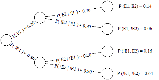
Figure 1: A Bayesian Network showing the probability of rain
One attraction of Bayesian Networks is the efficiency that only one branch of the tree needs to be traversed. We are really only concerned with P(E1), P(E2|E1) and P(E2,E1).
We can also utilize the graph both visually and algorithmically to determine which parameters are independent of each other. Instead of calculating four joint probabilities, we can use the independence of the parameters to limit our calculations to two. It is self-evident that the probabilities of rain on the second day having rained on the first are completely autonomous from the probabilities of rain on the second day having not rained on the first.
At the same time as emphasizing parametric indifference, Bayesian Networks also provide a parsimonious representation of conditionality among parametric relationships. While the probability of rain today and the probability of rain tomorrow are two discrete events (it cannot rain both today and tomorrow at the same time), there is a conditional relationship between them (if it rains today, the lingering weather systems and residual moisture are more likely to result in rain tomorrow). For this reason, the directed edges of the graph are connected to show this dependency.
Friedman and Goldszmidt suggest looking at Bayesian Networks as a "story". They offer the example of a story containing five random variables: "Burglary", "Earthquake", "Alarm", "Neighbour Call", and "Radio Announcement".[11] [12] In such a story, "Burglary" and "Earthquake" are independent, and "Burglary" and "Radio Announcement" are independent given "Earthquake." This is to say that there is no event which effects both burglaries and earthquakes. As well, "Burglary" and "Radio Announcements" are independent given "Earthquake"--meaning that while a radio announcement might result from an earthquake, it will not result as a repercussion from a burglary.
Because of the independence among these variables, the probability of P(A,R,E,B) (The joint probability of an alarm, radio announcement, earthquake and burglary) can be reduced from:
P(A,R,E,B)=P(A|R,E,B)*P(R|E,B)*P(E|B)*P(B)
involving 15 parameters to 8:
P(A,R,E,B) = P(A|E,B)*P(R|E)*P(E)*P(B)
This significantly reduced the number of joint probabilities involved. This can be represented as a Bayesian Network:
![--[The conditional probabilities of an alarm giving the independent events of a burglary and earthquake]--](/sites/default/files/bayes35.gif)
Figure 2: The conditional probabilities of an alarm given the independent events of a burglary and earthquake.
Using a Bayesian Network offers many advantages over traditional methods of determining causal relationships. Independence among variables is easy to recognize and isolate while conditional relationships are clearly delimited by a directed graph edge: two variables are independent if all the paths between them are blocked (given the edges are directional). Not all the joint probabilities need to be calculated to make a decision; extraneous branches and relationships can be ignored (One can make a prediction of a radio announcement regardless of whether an alarm sounds). By optimizing the graph, every node can be shown to have at most k parents. The algorithmic routines required can then be run in O(2kn) instead of O(2n) time. In essence, the algorithm can run in linear time (based on the number of edges) instead of exponential time (based on the number of parameters).[12] [13]
Associated with each node is a set of conditional probability distributions. For example, the "Alarm" node might have the following probability distribution:[13] [14]
| E | B | P(A | E,B) | P(!A|E,B) |
|---|---|---|---|
| E | B | 0.90 | 0.10 |
| E | !B | 0.20 | 0.80 |
| !E | B | 0.90 | 0.10 |
| !E | !B | 0.01 | 0.99 |
For example, should there be both an earthquake and a burglary, the alarm has a 90% chance of sounding. With only an earthquake and no burglary, it would only sound in 20% of the cases. A burglary unaccompanied by an earthquake would set off the alarm 90% of the time, and the chance of a false alarm given no antecedent event should only have a probability of 0.1% of the time. Obviously, these values would have to be determined a posteriori.
Bayesian networks are useful for both inferential exploration of previously undetermined relationships among variables as well as descriptions of these relationships upon discovery. In the former case, raw computational power can be brought to bear upon a problem. In the case of determining the likelihood of rain the next day following a rainy day, raw meteorological data can be input into the computer and the computer can determine the resultant probability network. This process of network discovery is discussed by Friedman & Goldszmidt[14] [15]. Such a process is computationally intensive and NP-hard in its algorithmic implications. The benefit of such a process is evident in the ability to describe the discovered network in the future. The calculation of any probability branch of the network can then be computed in linear time.
The National Aeronautic and Space Administration has a large investment in Bayesian research. NASA's Ames Research Center is interested in deep-space exploration and knowledge acquisition. In gathering data from deep-space observatories and planetary probes, an apriori imposition of structure or pattern expectations is inappropriate. Researchers do not always know what to expect or even have hypotheses for which to test when gathering such data. Bayesian inference is useful because it allows the inference system to construct its own potential systems of meaning upon the data. Once any implicit network is discovered within the data, the juxtaposition of this network against other data sets allows for quick and efficient testing of new theories and hypotheses.
The AutoClass project is an attempt to create Bayesian applications that can automatically interpolate raw data from interplanetary probes, and deep space explorations.[15] [16] A graphical example of AutoClass's capabilities is displayed in Figure 3. Incidentally, the source code for AutoClass is available in both LISP and C on an Open Source basis.
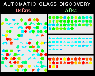
Figure 3: An AutoClass interpolation of raw data with no predefined categories. Sorted data is grouped by colour and shape. The top area is sorted into green-blue shapes, the middle into blues, and the bottom into red-orange-yellow shapes.
An applied example of AutoClass's capabilities was the input of infrared spectra. Although no differences among this spectra were initially suspected, AutoClass successfully distinguished two subgroups of stars.[16] [17]
Searching for a solution to a problem is usually an NP-hard problem resulting in a combinatorial explosion of possible solutions to investigate. This problem is often ameliorated through the use of heuristics, or sub-routines to make "intelligent" choices along the decision tree. An appropriately defined heuristic can quicken the search by eliminating obviously unsuccessful paths from the search tree. An inappropriately defined heuristic might eliminate the successful solutions and result in no evident solution.
Bayesian networks can replace heuristic methods by introducing a method where the probabilities are updated continually during search.
One class of search algorithms called Stochastic searching utilizes what are known as "Monte-Carlo" procedures. These procedures are non-deterministic and do not guarantee a solution to a problem. As such they are very fast, and repeated use of these algorithms will add evidence that a solution does not exist even though they never prove that such a solution is non-existent.
"Coupling such procedures with knowledge of properties of the distribution from which problem instances are drawn may be an effective way of extending the utility of these algorithms"[17] [18] by helping to focus in on areas of the search tree not previously studied.
Microsoft began work in 1993 on Lumiere, its project to create software that could automatically and intelligently interact with software users by anticipating the goals and needs of these users.
This research was in turn based on earlier research on pilot-aircraft interaction.[18] [20] The concern of this investigation was the ability of a system to supply a pilot with information congruent with the pilot's current focus of attention. Extraneous information or information not related to the pilot's current task list was suppressed.
"This ability to identify a pilot's focus of attention at any moment during a flight can provide an essential link to the provision of effective decision support. In particular, understanding the current goals of a pilot decision maker can be applied to select the presentation of alternative systems and displays."[19] [21]
The Lumiere project at Microsoft eventually resulted in the "Office Assistant" with the introduction of the Office 95 suite of desktop products.[20] [22]
In spite of their remarkable power and potential to address inferential processes, there are some inherent limitations and liabilities to Bayesian networks.
In reviewing the Lumiere project, one potential problem that is seldom recognized is the remote possibility that a system's user might wish to violate the distribution of probabilities upon which the system is built. While an automated help desk system that is unable to embrace unusual or unanticipated requests is merely frustrating, an automated navigation system that is unable to respond to some previously unforeseen event might put an aircraft and its occupants in mortal peril. While these systems can update their goals and objectives based on prior distributions of goals and objectives among sample groups, the possibility that a user will make a novel request for information in a previously unanticipated way must also be accommodated.
Two other problems are more serious. The first is the computational difficulty of exploring a previously unknown network. To calculate the probability of any branch of the network, all branches must be calculated. While the resulting ability to describe the network can be performed in linear time, this process of network discovery is an NP-hard task which might either be too costly to perform, or impossible given the number and combination of variables.
The second problem centers on the quality and extent of the prior beliefs used in Bayesian inference processing. A Bayesian network is only as useful as this prior knowledge is reliable. Either an excessively optimistic or pessimistic expectation of the quality of these prior beliefs will distort the entire network and invalidate the results. Related to this concern is the selection of the statistical distribution induced in modelling the data. Selecting the proper distribution model to describe the data has a notable effect on the quality of the resulting network.
These concerns aside, Bayesian networks have incredible power to offer assistance in a wide range of endeavours. They support the use of probabilistic inference to update and revise belief values. Bayesian networks readily permit qualitative inferences without the computational inefficiencies of traditional joint probability determinations. In doing so, they support complex inference modelling including rational decision making systems, value of information and sensitivity analysis. As such, they are useful for causality analysis and through statistical induction they support a form of automated learning. This learning can involve parametric discovery, network discovery, and causal relationship discovery.[21] [23]
In this paper, we discussed the premises of Bayesian networks from Bayes' Theorem and how such Bayesian inference differs from classical treatments of statistical inference. The reasons, implications and emerging potential of Bayesian networks in the area of Artificial Intelligence were then explored with an applied focus profiling some current areas where Bayesian networks and models are being employed to address real-life problems. Finally, we examined some of the limitations of Bayesian networks.
At best, such a paper can only be a snapshot of the state of Bayesian research at a given time and place. The breadth and eclectic foci of the many individuals, groups and corporations researching this topic makes it one of the truly dynamic areas within the discipline of Artificial Intelligence.
[1] [24]Hopkins, K.D. & G.V. Glass. Basic Statistics for the Behavioral Sciences. Prentice-Hall Inc., Englewood Cliffs, N.J. 1978. p. 3.
[2] [25]Although this is properly a binomial distribution rather than a normal one, the use of [sigma] to represent the variability of the sample illustrates the basic point.
[3] [26]cf. Hopkins & Glass, p. 401ff for an example.
[4] [27]Stutz, J. & P. Cheeseman, "A Short Exposition on Bayesian Inference and Probability." June 1994. National Aeronautic and Space Administration Ames Research Centre: Computational Sciences Division, Data Learning Group.
[5] [28]Morgan, Bruce W. An Introduction to Bayesian Statistical Decision Processes. Prentice-Hall Inc., Englewood Cliffs, N.J. 1968. p. 15.
[6] [29]Friedman, N. & M. Goldszmidt, "Learning Bayesian Network from Data." SRI International. 1998. http://www.erg.sri.com/people/moises/tutorial/index.htm [30]
[7] [31]Heckerman, D. & D. Geiger. "Learning Bayesian Networks. Microsoft Research: Redmond WA. December 1994. p. 3. http://www.research.microsoft.com/research/dtg/heckerma/TR-95-02.htm [32]
[8] [33]Heckerman & Geiger. p. 3.
[9] [34]Heckerman & Geiger. p. 3.
[10] [35]Winkler, Robert L. An Introduction to Bayesian Inference and Decision. Holt, Rinehart and Winston, Onc., Toronto. 1972.
[11] [36]Friedman & Goldszmidt, http://www.erg.sri.com/people/moises/tutorial/sld009.htm [37]
[12] [38]Friedman & Goldszmidt, http://www.erg.sri.com/people/moises/tutorial/sld016.htm [39]
[13] [38]Friedman & Goldszmidt, http://www.erg.sri.com/people/moises/tutorial/sld020.htm [40]
[14] [41]Friedman & Goldszmidt, http://www.erg.sri.com/people/moises/tutorial [42]
[15] [43] Stutz, J., W. Taylor & P. Cheeseman
"AutoClass C - General Information" NASA, Ames Research Center: 1998. http://ic-www.arc.nasa.gov/ic/projects/bayes-group/autoclass/autoclass-c-program.html#AutoClass C [44]
[16] [45] http://ic-www.arc.nasa.gov/ic/projects/bayes-group/autoclass/index.html [46]
[17] [47]Stewart, H. & Masjedizadeh, N.
"Bayesian Search" NASA, Ames Research Center: 1998. http://ic.arc.nasa.gov/ic/projects/bayes-search.html [48]
[18] [49] Cooper, G., E. Horvitz, & R. Curry
"Conceptual Design of Goal Understanding Systems: Investigation of Temporal Reasoning Under Uncertainty" Decision Theory & Adaptive Systems Group, Microsoft Research. Microsoft Corp. Redmond, WA: 1998. http://research.microsoft.com/research/dtg/horvitz/goal.htm [50]
[19] [51] Horvitz, E.
"Lumiere Project: Bayesian Reasoning for Automated Assistance" Decision Theory & Adaptive Systems Group, Microsoft Research. Microsoft Corp. Redmond, WA: 1998. http://research.microsoft.com/research/dtg/horvitz/lum.htm [52]
[20] [53] Heckerman, D. & E. Horvitz
"Inferring Informational Goals from Free-Text Queries: A Bayesian Approach" Decision Theory & Adaptive Systems Group, Microsoft Research. Microsoft Corp. Redmond, WA: 1998. http://research.microsoft.com/research/dtg/horvitz/aw.htm [54]
[21] [55] http://www.erg.sri.com/people/moises/tutorial/sld029.htm [56]
Links
[1] https://niedermayer.ca/node/31#fn0
[2] https://niedermayer.ca/node/31#fn1
[3] https://niedermayer.ca/node/31#fn2
[4] https://niedermayer.ca/node/31#fn3
[5] https://niedermayer.ca/user/login?destination=node/33%23comment-form
[6] https://niedermayer.ca/node/31#fn4
[7] https://niedermayer.ca/node/31#fn5
[8] https://niedermayer.ca/node/31#fn6
[9] https://niedermayer.ca/node/31#fn7
[10] https://niedermayer.ca/node/31#fn8
[11] https://niedermayer.ca/node/31#fn9
[12] https://niedermayer.ca/node/31#fn10
[13] https://niedermayer.ca/node/31#fn11
[14] https://niedermayer.ca/node/31#fn12
[15] https://niedermayer.ca/node/31#fn13
[16] https://niedermayer.ca/node/31#fn14
[17] https://niedermayer.ca/node/31#fn15
[18] https://niedermayer.ca/node/31#fn16
[19] https://niedermayer.ca/user/login?destination=node/37%23comment-form
[20] https://niedermayer.ca/node/31#fn17
[21] https://niedermayer.ca/node/31#fn18
[22] https://niedermayer.ca/node/31#fn19
[23] https://niedermayer.ca/node/31#fn20
[24] https://niedermayer.ca/node/21#fn0
[25] https://niedermayer.ca/node/21#fn1
[26] https://niedermayer.ca/node/21#fn2
[27] https://niedermayer.ca/node/33#fn3
[28] https://niedermayer.ca/node/34#fn4
[29] https://niedermayer.ca/node/25#fn5
[30] http://www.erg.sri.com/people/moises/tutorial/index.htm
[31] https://niedermayer.ca/node/25#fn6
[32] http://www.research.microsoft.com/research/dtg/heckerma/TR-95-02.htm
[33] https://niedermayer.ca/node/25#fn7
[34] https://niedermayer.ca/node/25#fn8
[35] https://niedermayer.ca/node/35$fn9
[36] https://niedermayer.ca/node/35#fn10
[37] http://www.erg.sri.com/people/moises/tutorial/sld009.htm
[38] https://niedermayer.ca/node/35#fn12
[39] http://www.erg.sri.com/people/moises/tutorial/sld016.htm
[40] http://www.erg.sri.com/people/moises/tutorial/sld020.htm
[41] https://niedermayer.ca/node/27#fn13
[42] http://www.erg.sri.com/people/moises/tutorial
[43] https://niedermayer.ca/node/36#fn14
[44] http://ic-www.arc.nasa.gov/ic/projects/bayes-group/autoclass/autoclass-c-program.html#AutoClass C
[45] https://niedermayer.ca/node/36#fn15
[46] http://ic-www.arc.nasa.gov/ic/projects/bayes-group/autoclass/index.html
[47] https://niedermayer.ca/node/37#fn16
[48] http://ic.arc.nasa.gov/ic/projects/bayes-search.html
[49] https://niedermayer.ca/node/38#fn17
[50] http://research.microsoft.com/research/dtg/horvitz/goal.htm
[51] https://niedermayer.ca/node/38#fn18
[52] http://research.microsoft.com/research/dtg/horvitz/lum.htm
[53] https://niedermayer.ca/node/38#fn19
[54] http://research.microsoft.com/research/dtg/horvitz/aw.htm
[55] https://niedermayer.ca/node/30#fn20
[56] http://www.erg.sri.com/people/moises/tutorial/sld029.htm